Improve spaCy's NER performance through uncertainty

Published Jul 31, 2020

🇫🇷 Lire en français

In this article, we will see how the search for uncertainty of a fairly complex model enables to substantially increase accuracy as well as end user satisfaction with a supervised learning system.

The topics will be detailed in the following order: context and first adopted solution, choice of model NER (Named Entity Recognition), error analysis and uncertainty quantification to improve results. The presented data are fake for confidentiality reasons.

Introduction

In a recent project, my goal was to extract information from a PDF corpus. After reading a dozen documents quickly, it turned out that several searched fields followed a fairly simple recurring pattern. This allowed the creation of a very simple first model based on regular expression . The following elementary pipeline validates 70% objectives:

Convert PDF to text file with pdftotext
Perform some cleaning tasks (special characters, lemmatization)
Search recurring patterns (e.g. “closing date:”)
Extract the entity of interest that follows the pattern:
1. Either with a regular expression (for a date contained in the text variable: re.findall(r'(\d+/\d+/\d+)', text))
2. Or with a lookup table (search for a match between the table and the N characters following the pattern)

To create a first view of this pipeline, I chose streamlit - a project which allows to quickly create a rendering in the browser. The few lines of code below display a page where a PDF can be uploaded and the model result be seen.

import streamlit as st

st.title('Extracteur d\'information')
pdf_file = st.file_uploader('', type=['pdf'])
show_file = st.empty()
if not pdf_file:
    show_file.info('Sélectionnez un PDF à traiter.')

base64_pdf = base64.b64encode(pdf_file.read()).decode('utf-8')
pdf_display = f'<embed src="data:application/pdf;base64,{base64_pdf}" width="700" height="1000" type="application/pdf">'
st.markdown(pdf_display, unsafe_allow_html=True)

pdf_text = _convert_pdf_to_text_and_clean(pdf_file)
predictions = _run_model(pdf_text)

show_file.info(f"""Titre : {predictions['title']}
                   Date : {predictions['date']}""")
pdf_file.close()

Figure 1: Streamlit application

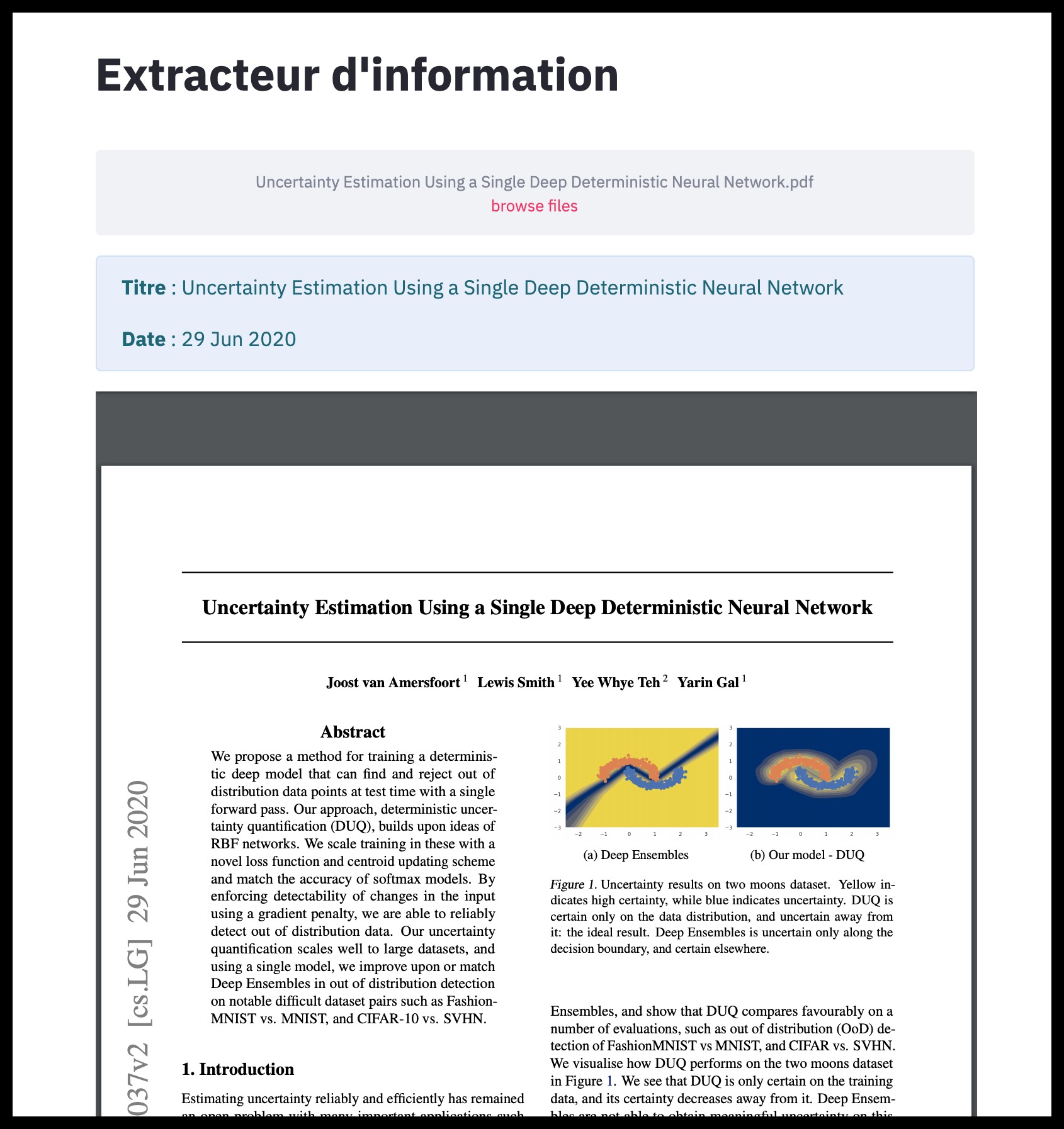Figure 2: PDF and predictions preview

In addition to make the task easy, the streamlit community is active (see the resolution of the PDF rendering issue .

The two conclusions of this first part have - for my greatest happiness - become prosaic: at the beginning of project, the most value are produced by the most naive ideas and the open source tools are admirable.

The NER model

Some fields are more complex to extract. A simple statistical analysis is not sufficient to find recurring patterns. They are neither in a defined place in the text nor have any particular structure. Some internet research quickly lead us to named entity recognition models NER which allow to associate words with labels thanks to supervised learning.

Several libraries implement easy to use wrappers for training and inference. I chose spaCy which highlights its ergonomics and temporal performances (~2 hours per training on a 16-core CPU). For more details on how the model works, the documentation, especially this video is useful.

The dataset contains 3,000 partially annotated documents. Partially means that all the searched fields are not annotated, however when a field is annotated, it is over the entire dataset. The annotation has been done automatically by scrapping the HTML code of web pages. For the cross-validation strategy the data has been splitted as follow: 2,100 documents for the training and 900 for the validation. The required accuracy is 95% for each field.

The following is an example of the expected input format:

TRAIN_DATA = [
    ("Horses are too tall and pretend to care about your feelings",
     {"entities": [(0, 6, "ANIMAL")]}),
    ("Who is Shaka Khan?",
     {"entities": [(7, 17, "PERSON")]}),
    ("I like London and Berlin.",
     {"entities": [(7, 13, "LOC"), (18, 24, "LOC")]}),
]

Note that each example consists of a text followed by its label delimited by two numbers: start and end indices. PDFs in our database yield texts that are too large to fit in RAM. A handy tip is to split the text into chunks. Nevertheless it creates lots of examples without labels (many chunks have no entity of interest). The dataset is said to be sparse. A rebalancing function overcomes this problem by selecting a sample without label with a fairly weak probability.

def _balance(data):
    balanced_data = [row for row in data if len(row[1]['entities']) > 0 or np.random.rand() < .1]
    return balanced_data

The probability 0.1 can be adjusted, the objective being to reach a reasonable proportion of sample with label (50% in our case). The algorithm thus sees many examples without annotation but is not saturated with these.

Once the data is formatted, reading the example scripts provided allows to start training a first model. I made some preliminary changes to the code:

refactor and test the code
use click for the command lines
add tqdm to monitor time-consuming tasks
create a function to compute our own business metric at each iteration (by default only the loss is calculated)

Let’s take a closer look at this metric. To assess the results, we first restrict ourselves to a single field (for example the title of the document). What interests our user is the field regardless of the number of times it appears or its position in the PDF (see Fig. 2). Our prediction will thus be a majority vote per document. If the model predicts “[a, a, b]” to be titles, the final prediction will be “a”. Remember that the goal is to achieve 95% correct answers.

The first training yielded a 67% benchmark. After splitting the texts into pieces, the algorithm reaches 72%. Finally, the rebalancing saves 4 more points to reach 76% accuracy.

Error analysis

A crucial step in inferential statistics is the study of errors. This analysis has a double virtue: better understand the model and focus on its weaknesses to improve it. Let’s take a look at the PDFs whose title has not been found to attempt to investigate the causes of these blunders.

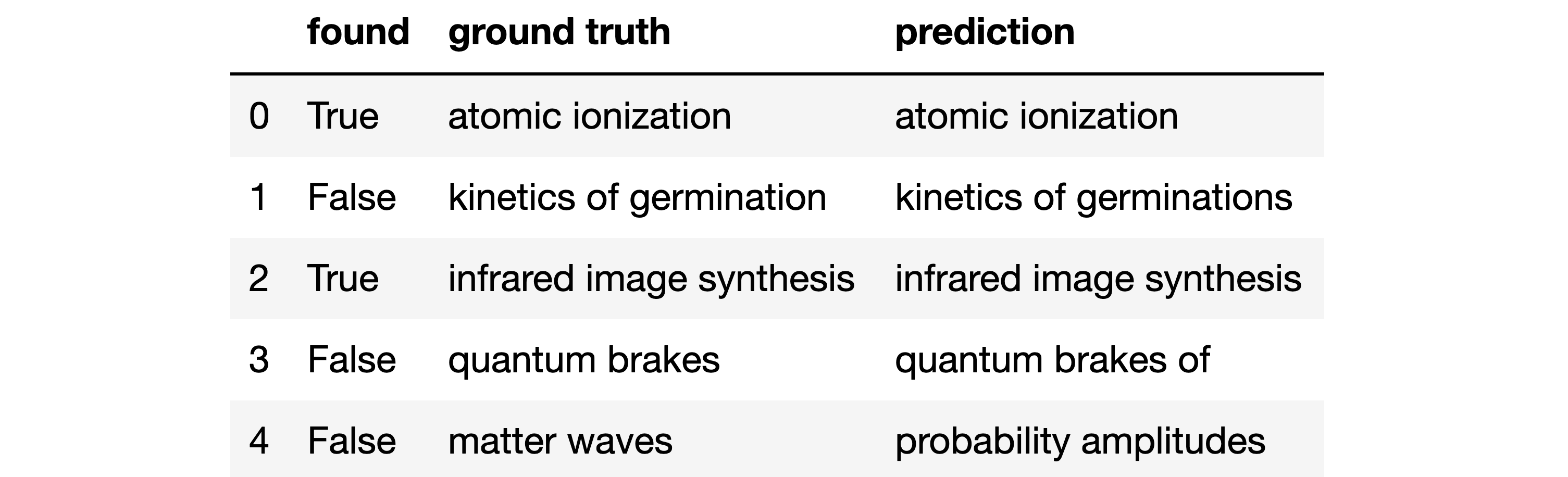Figure 3: Error analysis

We want to focus on errors, i.e. when the found column is False. There are 3 errors in the table above:

Index 4: nothing in common between the prediction and the real value
Index 3: more subtle error, the word “of” must not appear
Index 1: even closer, there is an extra “s”

After a review with the client, it seems that little mistakes don’t matter. We can therefore build a distance which allows to be more flexible on the acceptance of the prediction. The function below checks that the predicted value is not empty, then accepts the result if it is included in the ground truth or if the Levenshtein distance is less than 5 (arbitrarily chosen value).

from Levenshtein import distance

def flexible_accuracy(x):
    pred, gt = x['prediction'], x['ground truth']
    return True if pred and distance(pred, gt) < 5 and (gt in pred or pred in gt) else False

df.apply(flexible_accuracy, axis=1).mean()

Without having changed anything in the model, we reach an accuracy of 82% for our users. There is still a way to go but a few points were won without effort.

Quantify uncertainty

At this level of the project, improvements are less obvious. For the brevity of the article, I will not focus on the unsuccessful or less successful trials, among which we find: work on data and re-training with updated hyperparameters.

To continue on the error analysis, I wanted to quantify the uncertainty of predictions. The ease of use of spaCy has a cost, we discover it when trying to access probabilities. Nevertheless, knowledge sharing within the community again allows to find a clue:

def _predict_proba(text_data, nlp_model):
    proba_dict = defaultdict(list)
    for text in text_data:
        doc = nlp_model(text)
        beams = nlp_model.entity.beam_parse([doc], beam_width=16, beam_density=0.0001)
        for beam in beams:
            for score, ents in nlp_model.entity.moves.get_beam_parses(beam):
                for start, end, label in ents:
                    proba_dict[doc[start:end].text].append(round(score, 3))
    return dict(proba_dict)

This function returns a confidence score between 0 and 1 for each group of words identified as being a title.

{"the real doc title": [1.0, 0.946, 1.0, 0.3], 
 "a semblance of title": [0.123, 0.356, 0.65], 
 "any words": [0.006],
 "something else": [0.981]}

For more clarity we aggregate by summing the confidences, we normalize by dividing by the total sum and we sort in descending order. Standardization makes it possible to compare the confidences between documents.

{"the real doc title": 0.605,
 "a semblance of title": 0.211,
 "something else": 0.183,
 "any words": 0.001}

We naturally consider the word group with the greatest confidence to be the best prediction. Let’s plot the density of good and bad predictions according to the uncertainty.

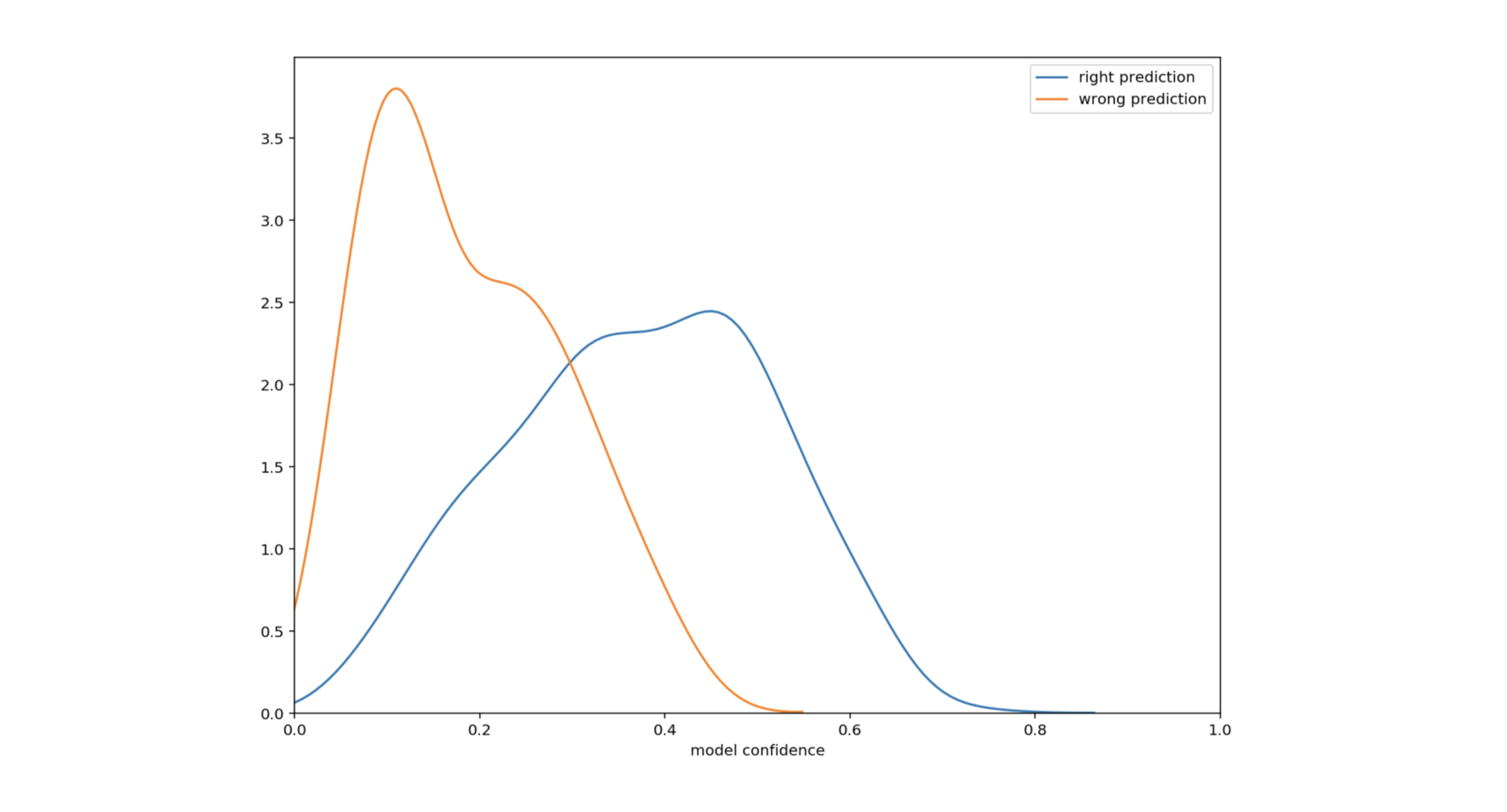Figure 4: Density of predictions as a function of uncertainty

This plot shows that the uncertainty is smaller when the predictions are correct. Especially for a confidence greater than 0.4 (39% of cases), the accuracy is 99%. Maybe this is a way to increase our performance. Let’s focus on confidences below 0.4 (61% of cases). Below this threshold, the accuracy drops to 72%. A careful analysis of these weak confidences reveals that for the 28% of error cases, the value with the second highest confidence is often the correct one. This is true 62% of the time. In other words, in 62% of error cases - representing 28% of low confidence cases - the right answer is the second choice.

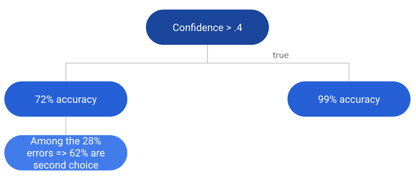Figure 5: Summary in tree form

There is no injunction to use the pure response of our model. The best algorithm is the one which is best aligned with the user need. It turns out here that the user favors accuracy. We therefore propose a rule based on Fig. 5 which returns the prediction when the confidence is greater than the threshold, otherwise, it yields the two predictions with the highest confidence.

We can calculate the accuracy with which the user will see the correct answer among those proposed:

\[\begin{eqnarray} Accuracy_{Conf<0.4} &=& Accuracy_{FirstChoice} + Accuracy_{SecondChoice} \\ &=& 0.72 + (1-0.72) * 0.62 \\ &=& 0.89 \\ \end{eqnarray}\] \[\begin{eqnarray} FinalAccuracy &=& 0.39 * Accuracy_{Conf>0.4} + (1-0.39) * Accuracy_{Conf<0.4} \\ &=& 0.39 * 0.99 + 0.61 * 0.89 \\ &=& 0.93 \\ \end{eqnarray}\]

93% accuracy is achieved. To be more rigorous, a disjoint validation set should be created to check this performance.

Conclusion

The goal is not quite reached but the gain is substantial. Vincent Warderdam recalls lucidly in this presentation that it is sane to “predict less but carefully”. Using uncertainty information is beneficial in plenty of use cases. The conditions must simply be validated by the user. For example, it would not have been suitable in our example to give the 5 highest confident predictions because the user would have had too much information to process.

The transparency of the uncertainty of the model is undoubtedly a lever to increase the user satisfaction. The imperfections of an algorithm must be exhibited to gain the trust of users.

Key takeaways:

Start simple with a short feedback loop: what can be done without supervised learning?
Adapt and relax the model and the metric to the use case
Use uncertainty:
1. focus on the most uncertain cases
2. let the users know when the model is not confident

To go further:

Find the minimal number of data from which the spaCy model converges (to add new fields in the app)
Try to improve performance by averaging with another NER model like huggingface or allennlp when confidence is low
Analyse the errors from the a data perspective: sampling issues for low confidences?