Probability calibration
I gave a talk on this topic at the PyData NYC 2019. Video can be found here
In the previous article, we described a technique to measure the
uncertainty in regression.
What about the other supervised learning field: classification?
It is very useful to be able to control the level of confidence in the predictions of models. For exemple, in the classical binary classification example of malignant/benign tumors, we would like to affirm that if the probability is 0.3, there is indeed a 30% risk that the tumor is malignant. This is far from being the case in practice for many algorithms.
Below are two examples where having a calibrated probability is necessary:
-
In marketing, we evaluate what a client brings back throughout the period during which he remains loyal to the company: the Customer Lifetime Value (CLV). It is then common to multiply the price of a product by the probability that it has to be bought: $CLV = 200€\times0.1 = 20€$.
-
In medicine some results are sensitive. The order of probabilities of having cancer doesn’t matter to patients. In contrast, a probability with physical meaning is vital.
Uncalibrated models are a pain when it comes to interpreting the result of
predict_proba.
The abstraction of this method - which tend to be used without understanding of what is behind it - is very
dangerous when we see the calibration concerns that we will illustrate in the first part.
However, methods exist to overcome the pitfalls of calibration such as isotonic regression
which we will detail in the second part.
The code used is available here and there.
Calibration curves
Unlike regression which allows a continuous variable to be estimated, classification returns a probability of belonging to a class $C$. The target variable $Y$ is said to be discrete. We seek the conditional probability for $Y$ to belong to the class $C$ knowing $X$ (the explanatory variables):
\[P(Y=C|X)\]How do we interpret this probability?
Without dwelling on the epistemology of this term, let us note that it can mean both the chance that
an event has of being realized from a frequentist point of view, but also the degree of belief in the
realization of the event in the presence of uncertainty. For the sake of simplicity, we will confuse
these two concepts in the rest of this article.
Following our reasoning it is necessary to have well calibrated predicted probabilities to access the degree of uncertainty of our model. This means that the proportion of individuals with the same probability of belonging to a class is equal to this probability. As seen in the introduction, if we take all the individuals with a probability $P=0.3$ of belonging to the class $C=Malignant Tumor$, approximately 30% of them must actually have a malignant tumor.
However, most classifiers are rarely calibrated. There is a way to measure the quality of an estimator on this aspect: the calibration curve [1]. It is implemented in the scikit-learn library. The algorithm is as follows:
-
cut the [0, 1] axis into several intervals
-
select the individuals whose probability belongs to each interval
-
calculate the proportion of individuals belonging to class C
This code is used to generate Figures 1 and 2.
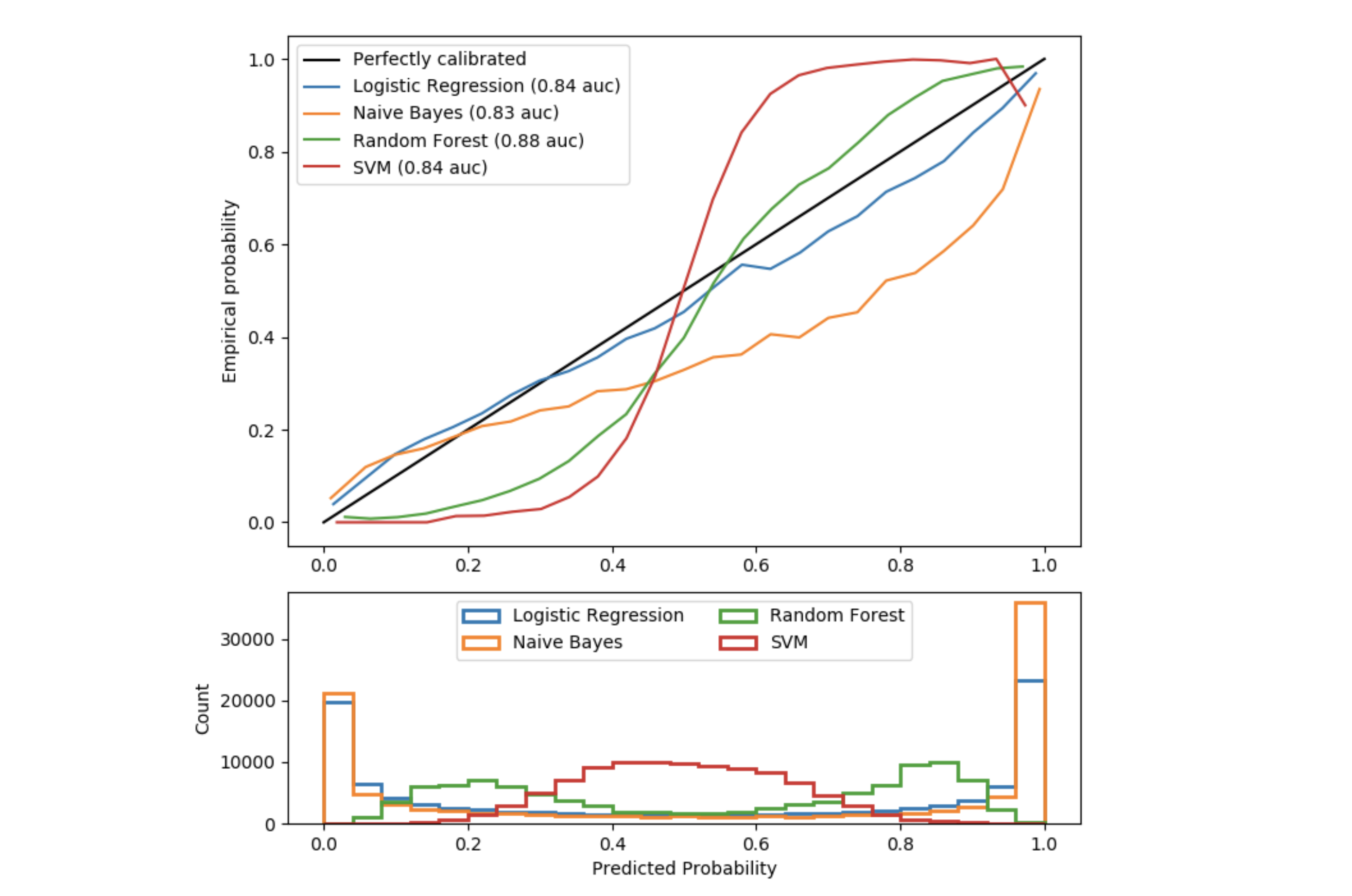 Figure 1: Calibration curves for 4 classifiers
This figure illustrates the pitfalls of the results of methods called predict_proba in classification algorithms. Data is simulated using the make_classification method and the classifiers have been set to have comparable auc score.
-
The black line represents the perfect calibration: for each group of individuals with a similar predicted probability, the proportion (empirical probability) of these individuals really being in class 1 is equal to the predicted probability.
-
Logistic Regression is the best calibrated model in this figure: it is close to the black line. This is indeed a special case of generalized linear models. A probability law (Bernoulli) is associated with the response $Y$. The model therefore gives probabilities in the statistical sense by construction hypothesis.
-
The Naive Bayes Classifier already sees its probabilities less well calibrated, especially those close to 1. In fact, this model returns many probabilities but the so-called «naive» hypothesis of independence of the explanatory variables is never respected in practice (2 variables are also redundant in the simulated data). The transposed sigmoid translates the over-confidence of the algorithm in its predictions. For individuals predicted at 0.8, only 50% actually belong to class 1.
-
The Random Forest shows a histogram with probability peaks at 0.2 and 0.8, while probabilities close to 0 or 1 are very rare. Indeed, the fact of averaging predictions of decision trees between 0 and 1 prevents finding extreme values (it would be necessary for all weak classifiers to agree on extreme values, which is very rare because of the bagging which creates noise). As a result, there is a sigmoid indicating that the classifier could trust his intuition more and bring the probabilities closer to 0 and 1.
-
The Support Vector Machine does not have a predict_proba method but a decision_function method which returns the distance to the separating hyperplane (i.e. decision boundary) as a confidence indication. This distance (not between 0 and 1) is not a probability and we can clearly see it by observing again a sigmoid even further from the black line.
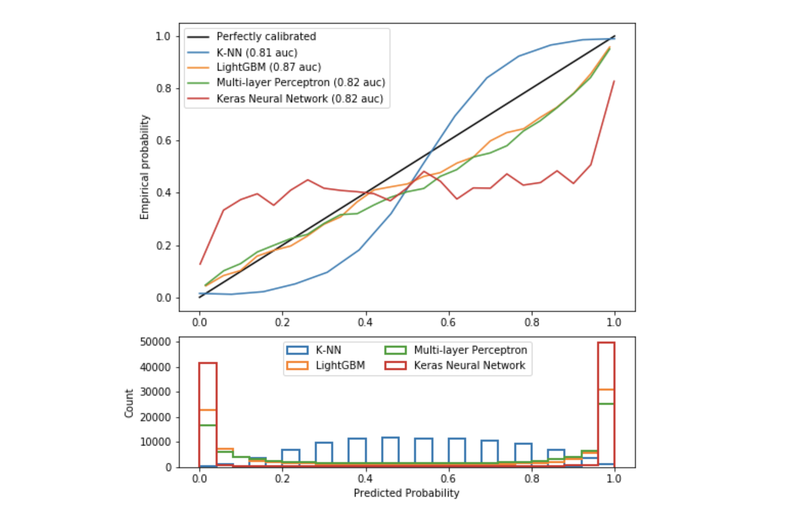 Figure 2: Calibration curves for 4 next classifiers
This second figure is similar to the first with other algorithms, the separation has been made for the sake of clarity.
-
The k-nearest neighbor algorithm again shows a sigmoid. Indeed the method predict_proba does not compute a probability. It is the mean of the nearest classes weighted by the inverse of the distance. For example, if $k=15$, twelve closest neighbors are 1 and three are 0, all being equidistant, then the probability of belonging to class 1 would be $\dfrac{12}{15}=0.8$.
-
The LightGBM algorithm is a boosting method. The probabilities aren’t bad due to the optimization of the logloss.
-
The perceptron is fairly well calibrated because it is made up of a single layer of 100 neurons. Thus, the learned function is linear. In addition, the output activation is a sigmoid, which approximates many probabilities.
-
The Keras neural network is made up of 2 layers, the architecture is more complex, the function is no longer linear. For several years now, the performance of networks has exploded, as has the complexity of their architectures. The techniques used to avoid the problems of vanishing gradient and ReLu dying [2] have degraded the calibration of probabilities [3].
N.B: Undersampling and oversampling techniques - to tackle the problem of unbalanced data - modify the prior distribution and generate very poorly calibrated probabilities.
How to avoid this recurring calibration problem?
Isotonic regression
An existing technique, the isotonic regression initially proposed in [4], is based on the following principle:
-
Train a classification model
-
Plot the calibration curve
-
If the probabilities are not calibrated, train an isotonic regression with input $X$: the probabilities predicted by the classifier and with target $y$ the associated real targets
-
Compute the calibrated probabilities by composing the isotonic regression and the model: $p=IsotonicRegression(model(X))$
Here is an example of python code that calibrates the probabilities of a naive Bayesian classifier:
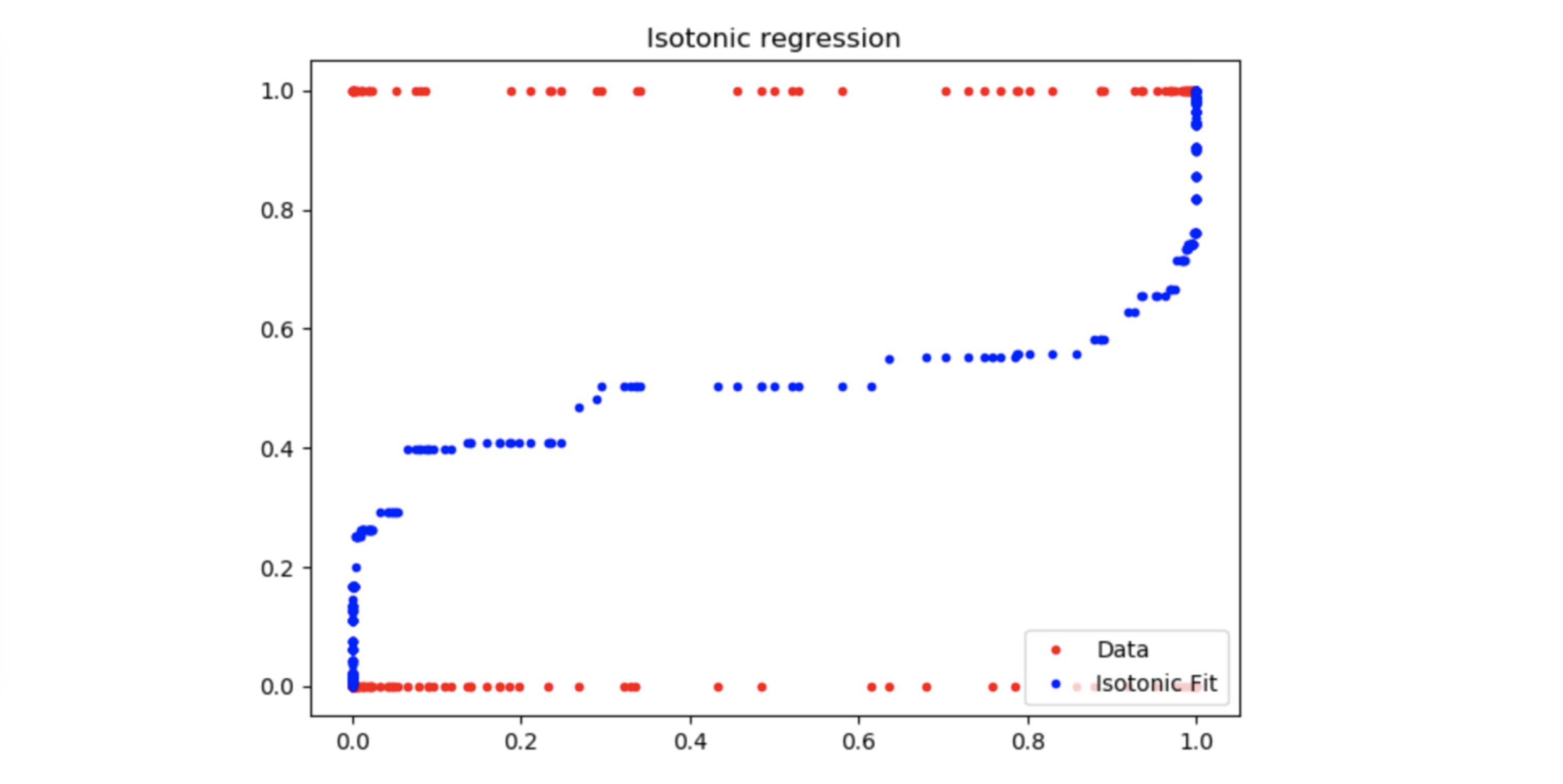 Figure 3: Isotonic regression
The resulting isotonic regression fits well with the calibration curve of the Naive Bayes Classifier in fig. 1. Thus, if the classifier returns an over-confident probability of 0.2, our calibrated model will return approximately a probability of 0.4 according to the blue curve above.
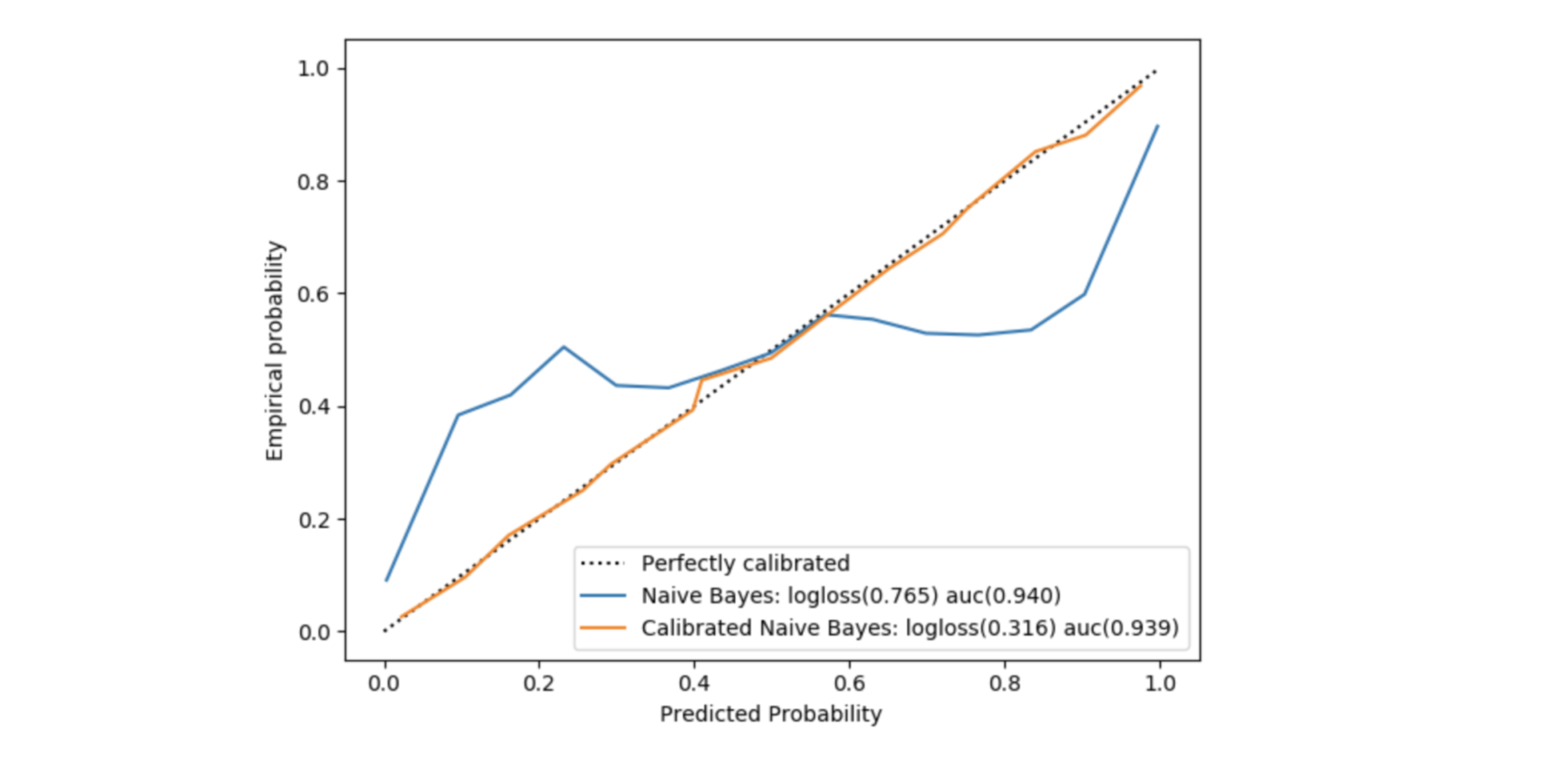 Figure 4: Comparison of probabilities before and after calibration
The CalibratedClassifierCV class allows you to do this concisely, but it seemed interesting to detail it in the code for the sake of understanding. In fig. 4, in addition to the calibration difference between the simple model and the calibrated one, we see that the logloss score is significantly better when the probabilities are calibrated (this is true only for models that do not directly optimize this cost function). On the other hand, the auc score is almost unchanged since this metric only depends on the order of probabilities and the isotonic regression has a monotonicity constraint.
Isotonic regression is a non-parametric, increasing function $f$, which transforms a vector of probabilities in a vector of calibrated probabilities such as $P_{calibrated}=f(P_{classifier})$.
Finding $f$ is to minimize the least squares while imposing a monotonicity constraint:
\[\min \sum_{i=1}^{n}(y_i - f(p_i))^2 \quad / \quad ∀ \quad p_i < p_j, \quad f(p_i) < f(p_j)\]The algorithm used - which we will only illustrate [5] - is called PAVA (Pool Adjacent Violators Algorithm) and has a linear complexity. It takes as input the vector of real targets ordered by increasing predicted probability.
This code snippet generates the following figure:
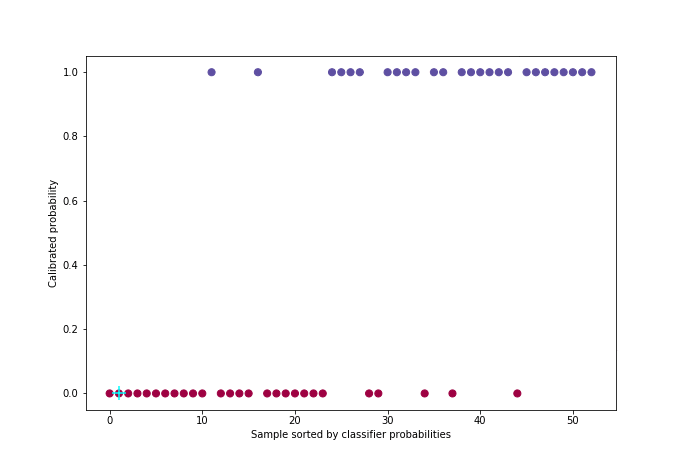 Figure 5: Calibration with PAVA algorithm
For better visualization, approximately 50 individuals were uniformly sampled from the probability distribution among the 21,000 in the cross-validation set.
This method has the advantage over others of properly calibrating the probabilities regardless of the calibration default of the classifier (over or under-confidence). On the other hand, the condition to work well is that one must have enough data since there are two learning stages, one for the classifier and one for the isotonic regression.
Conclusion
Key takeaways:
-
Estimating uncertainty is possible in classification: you should first check the quality of the probabilities and then calibrate them if necessary.
-
The calibration matches the output of predict_proba method with the physical intuition that we have of a probability, which allows us to adjust the actions to be taken according to the business case.
-
Models that do not optimize logloss or unbalanced data problems often give poorly calibrated probabilities.
-
For two models with equivalent score, we will prefer the one that has higher self-confidence when the probabilities are calibrated (i.e. the probabilities are close to 0 and 1).
To go further:
-
For multiclass classification, a possible approach is to consider the problem as several binary classifications.
-
Other methods exist:
-
Parametric algorithms (useful when too little data is available for non-parametric methods)
-
Fit a sigmoid for under-confident classifier (e.g. SVM)
-
Beta calibration for over-confident classifier (e.g. Naïve Bayes)
-
-
Non-parametric algorithms
-
An algorithm based on cubic splines which manages the multiclass case and can be smoother in the calibration compared to the isotonic regression which returns pieces of constant functions [6].
-
The Bayesian Binning [7] which tries to solve the problem of the possible non-monotony of the calibration curve.
-
-
-
Finally, bayesian learning, a popular subject, tackles neural networks and offers a new approach based on the notion of uncertainty. The TensorFlow Probability library offers the possibility of learning the parameters of distributions to predict this uncertainty.
Edit: I found an interesting paper that try to evaluate predictive uncertainty under dataset shift [8]. One conclusion is that improving calibration and accuracy on an in-distribution test set often does not translate to improved calibration on shifted data. I guess I’ll have to write a new article on how to get better uncertainty without calibration ¯\_(ツ)_/¯.
Références
[1] https://jmetzen.github.io/2015-04-14/calibration.html
[2] Dying ReLU and Initialization: Theory and Numerical Examples. Lu Lu, Yeonjong Shin, Yanhui Su, George Em Karniadakis. 2019
[3] On Calibration of Modern Neural Networks. Chuan Guo, Geoff Pleiss, Yu Sun, Kilian Q. Weinberger. 2018
[4] Transforming Classifier Scores into Accurate Multiclass Probability Estimates. Bianca Zadrozny and Charles Elkan. 2002
[5] http://fa.bianp.net/blog/2013/isotonic-regression/
[6] Spline-Based Probability Calibration. Brian Lucena. 2018
[7] Obtaining Well Calibrated Probabilities Using Bayesian Binning. Mahdi Pakdaman, Gregory F. Cooper, and Milos Hauskrecht. 2015
[8] Can You Trust Your Model’s Uncertainty? Evaluating Predictive Uncertainty Under Dataset Shift. Yaniv Ovadia, Emily Fertig, Jie Ren, Zachary Nado, D Sculley, Sebastian Nowozin, Joshua V. Dillon, Balaji Lakshminarayanan, Jasper Snoek. 2019