Prediction intervals
I gave a talk on this topic at the PyData NYC 2019. Video can be found here
In supervised learning, a regression model allows us to infer the value associated with a sample from examples. Typically, we try to predict the average behavior of a target variable $Y$ from the explanatory variables $X$ describing the observations. It is the conditional expectation of $Y$ given $X$:
\[E\left(Y \left\vert X \right. \right)\]Is it possible to get more information than the average behavior from a prediction model?
Can we quantify the error of our model in its predictions?
To show how we can answer these questions, we will use the data Superconductivty Data [1] identifying the critical temperature in Kelvin below which different materials become superconductive.
Here, the target variable $Y$ is the critical temperature (critical_temp). The explanatory variables $X$ define the atomic structure of the material.
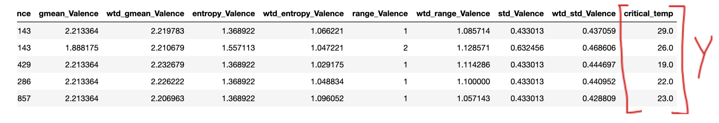 Figure 1: Superconductivity Data sample
Prediction intervals and confidence intervals should not be confused: the latter gives an interval for the conditional mean, taking into account only the sampling error, while the former takes also into account the error of the model versus the actual value.
Random Forest: From prediction to distribution
The Random Forest algorithm [2] is an aggregate of weak learners. In other words, we build many simple models (e.g. decision trees). The overall prediction of the algorithm is given by averaging the predictions of all trees.
A binary decision tree for regression is built with nodes (representing rules) on the explanatory variables. For example, is the average atomic mass of the observation less than 60u?
These rules are automatically defined by minimizing a cost function $J$. We minimize $J$ by calculating its value on different thresholds of different variables. By default, the scikit-learn library uses the mean squared error.
\[J = \frac{1}{n} \sum_{i=1}^{n}{(y_i - \widehat{y_i})^2}\]The minimization of this cost function gives an estimate of the conditional mean.
from sklearn.ensemble import RandomForestRegressor
rf = RandomForestRegressor(criterion='mse', n_estimators=1000, min_samples_leaf=1)
rf.fit(X_train, y_train)
first_tree = rf.estimators_[0]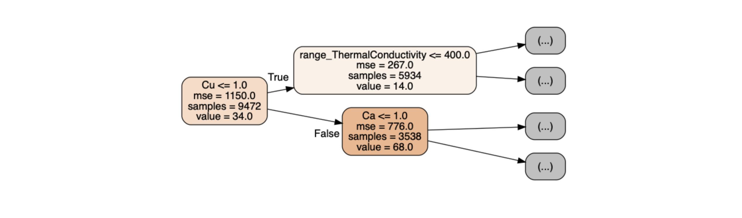 Figure 2: First nodes of the first tree of the forest
Fig. 2 illustrates the first three nodes of a decision tree:
-
range_ThermalConductivity <= 400 is the node rule associated with one variable.
-
mse is the value of the error, we see that it decreases as we go deeper in the tree.
-
samples is the number of observations passing through the node, we can check that 5934 + 3538 gives the number of initial observations 9472.
-
value is the average of the critical temperatures of the observations in the node (i.e: the prediction for this node).
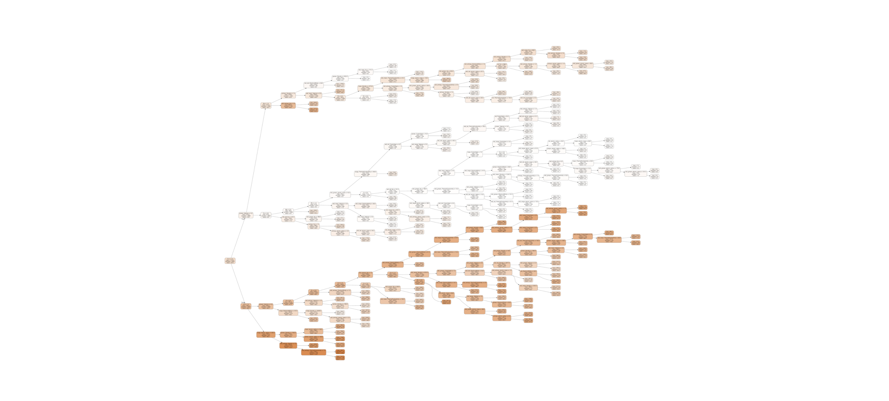 Figure 3: First tree of the forest
A decision tree is by default built until its leaves are pure (i.e. contain a single observation or several observations having the same critical temperature value). This corresponds to the min_samples_leaf=1 parameter in the code.
With this strategy, we can recover the predictions of each of the 1000 trees instead of keeping only the average value in order to get the whole distribution of predictions. The number of trees is defined by the parameter n_estimators.
We thus obtain an estimate of the conditional distribution, that associates for y ∈ R the probability for a given observation $X$ that its response $Y$ is less than $Y$:
\[y \rightarrow P\left(Y≤y \left\vert X=x \right. \right)\]decision_tree_predictions_matrix = np.transpose([decision_tree.predict(data_eval) for decision_tree in model.estimators_])This code returns the matrix of predictions for each tree for each observation. This allows us to plot Figure 5.
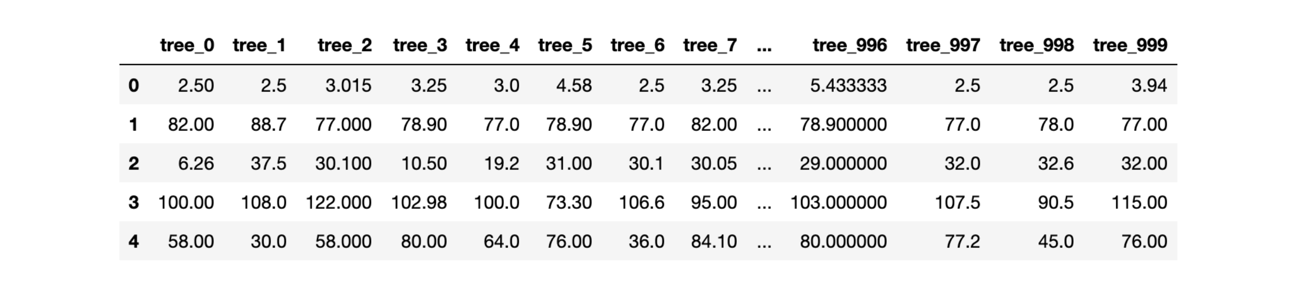 Figure 4: Prediction of each tree for material 0 to 4
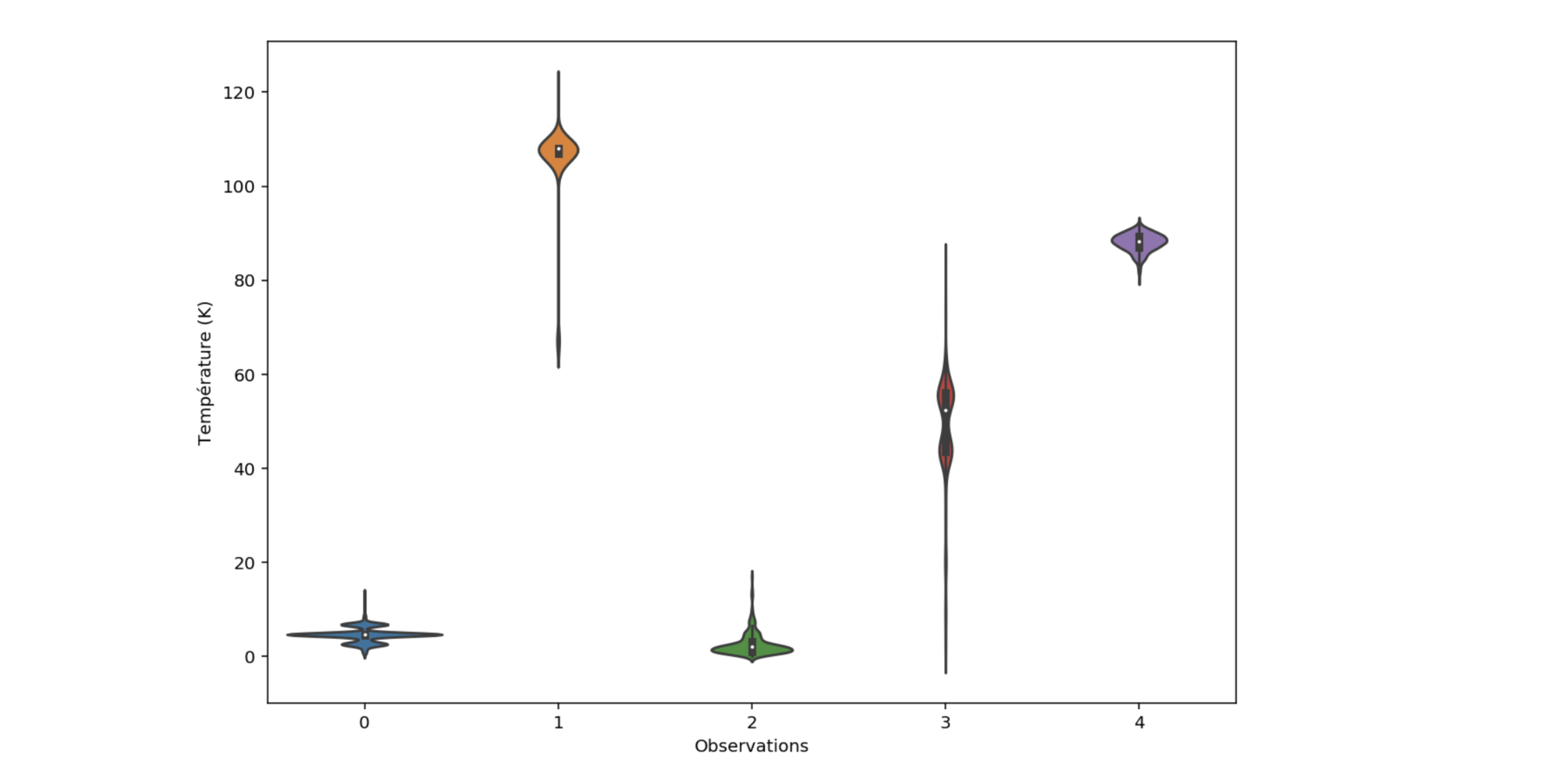 Figure 5: Predicted distribution for material 0 to 4
From the conditional distributions on each material, one can compute the mean (the value returned by the predict method of scikit-learn), but also the median, quantiles and other statistical moments.
The narrow distributions for observations 0, 2 and 4 show that the model seems more confident than its prediction in observations 1 and 3.
Quantify model confidence
We are particularly interested in the quantiles of the predicted conditional distributions. They make it possible to build prediction intervals for each material $x$.
\[I_{pred}(x) = [Q_{\alpha}(x), Q_{1-\alpha}(x)]\]By taking $\alpha$ equal to 0.05, $1-\alpha$ is worth 0.95. This means that we select the 5th and 95th percentiles from the predicted distribution of observation x. These two values form the prediction interval 90 (i.e. the interval which has a probability 0.9 of containing the true measured value of critical temperature for the material).
lower_bound_predictions = [np.percentile(prediction_distribution, 5) for prediction_distribution in decision_tree_predictions_matrix]
upper_bound_predictions = [np.percentile(prediction_distribution, 95) for prediction_distribution in decision_tree_predictions_matrix]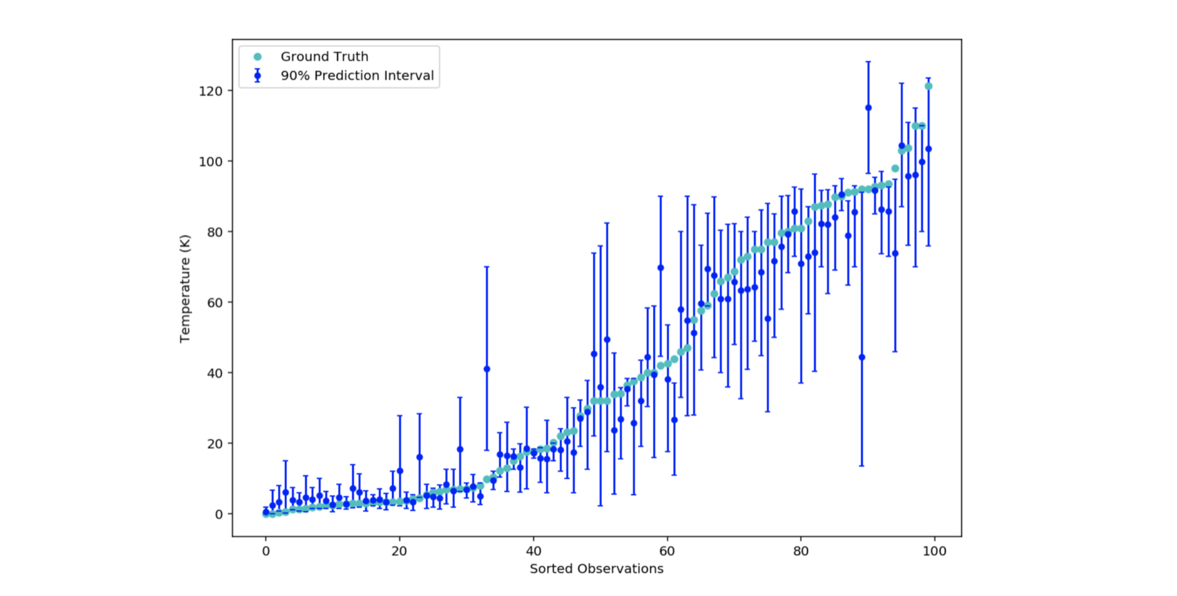 Figure 6: 90% prediction intervals of 100 materials
Let’s check that around 90% of the intervals contain the actual critical temperature value:
ground_truth_inside_interval = len([1 for i, value in enumerate(y_test) if lower_bound_predictions[i] <= value <= upper_bound_predictions[i]])
ground_truth_inside_interval_percentage = ground_truth_inside_interval / len(y_test)
That code returns 0.87, which means that 87 out of 100 intervals contain the real critical temperature value in fig. 6. The result seems consistent with the expected probability 0.9.
We thus have the possibility of quantifying how sure the model is of itself. The small prediction intervals to the left of fig. 6 (low temperature area) illustrate that percentiles 5 and 95 are close to each other. The weak learners predict roughly the same value. The model is robust for these observations. In contrast, for the right intervals, the variance seems much higher.
It is visually intuited that the predictions farthest from the actual critical temperature value are surrounded by a large interval. This can be checked by calculating the correlation coefficient between the error (of the conditional mean) and the size of the interval.
interval_length = upper_bound_predictions - lower_bound_predictions
absolute_error = abs(y_test - rf.predict(X_test))
correlation = np.corrcoef(interval_length, absolute_error)[0][1]
We find a strong positive correlation of 0.68 (strong because greater than 0.5) and significant because its associated p-value is less than 10-8.
Why is the model not confident in certain region
Let’s investigate: on fig. 6, high critical temperature prediction seem to have bigger intervals. Uncertainty can have two causes:
-
Aleatory variability: the natural randomness in a process (e.g. dice roll). This one is irreducible.
-
Epistemic Uncertainty: the scientific uncertainty in the modeling of the process. It is due to limited data and knowledge. This uncertainty can be reduced by better modeling or by adding relevant data.
Let’s focus on point 2. As we want to keep our model, we’ll dive into the limited data part. The distribution of the target variable in our dataset looks like this:
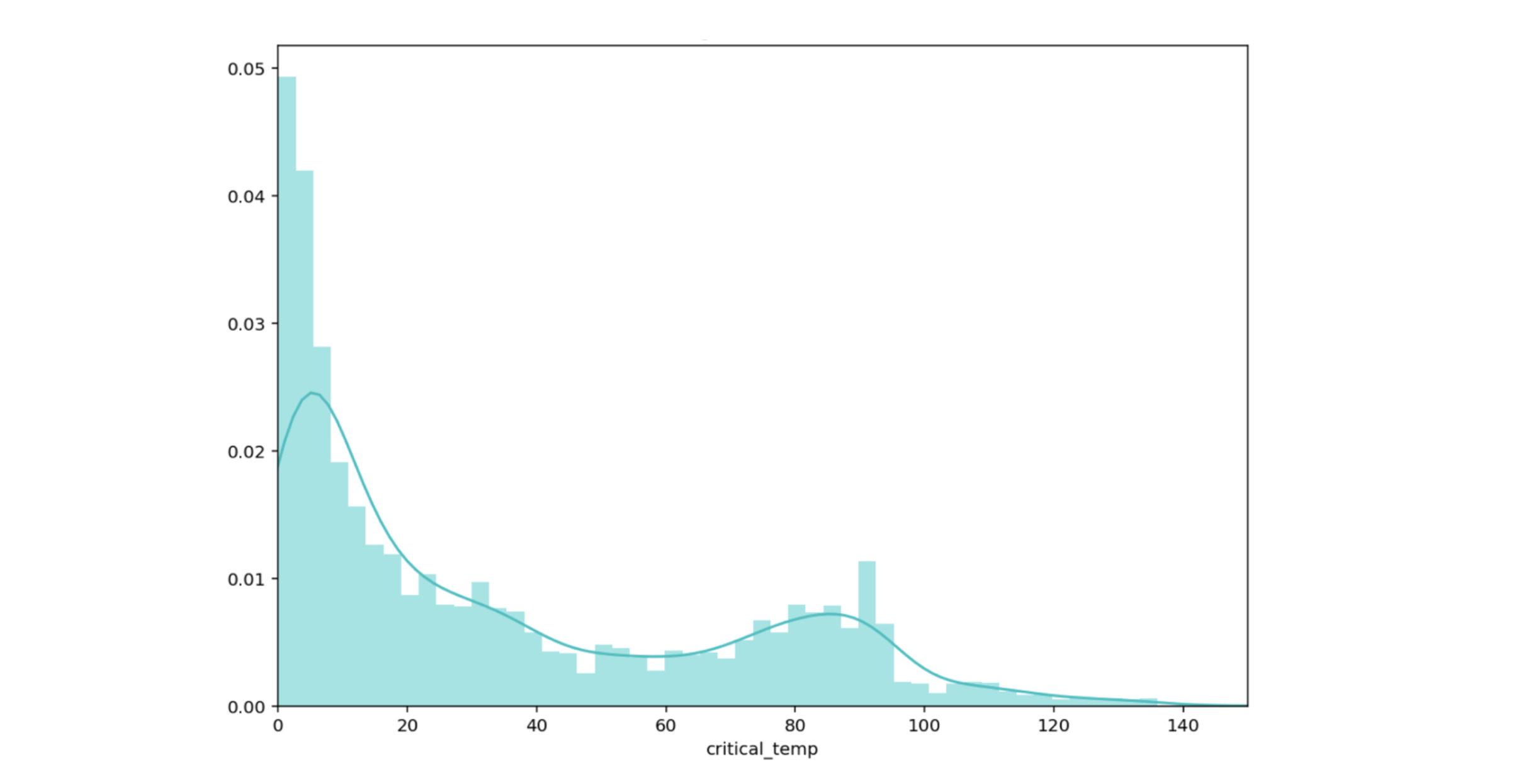 Figure 7: Critical temperature distribution
Most of the data is between 0 and 20K, with a second mode close to 80K. It is therefore not surprising that the model is more confident in the region of low temperatures.
How can this information help from a business point of view? I can see at least 3 reasons besides the fact that the information is inherent in the model (therefore free).
-
In a use case where the action to be taken is delicate (medicine, fraud, etc.), we will appreciate the measure of the uncertainty (no action if the prediction interval is too large - high risk).
-
As previously described, it provides rich information on the data used for training. A large prediction interval can indicate that few training samples are close to this region. It may make sense - if possible - to fetch more measure in these areas.
-
A very large interval may point out an outlier in the training data or an anomaly in the test data.
Generalization
Growing trees until the leaves are pure (as Breiman suggests [2]) does not always give optimum results depending on the metric chosen. You can adjust the min_samples_leaf parameter to reach better results.
Let’s set this parameter to 100 (the tree leaves will contain at least 100 observations) and examine the predicted distribution for one observation with a critical temperature of 72K.
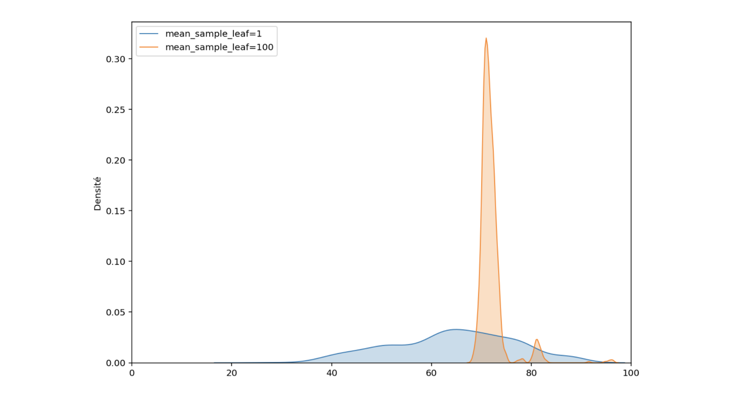 Figure 8: Comparison of the predicted distributions for one material
The orange distribution is narrower than the blue, the variance has decreased. In fact, by limiting the size of the trees, only the average of the critical temperatures falling in each leaf is kept. We no longer have the complete distribution of critical temperatures that were used for training, but only a distribution of sample means from these critical temperatures.
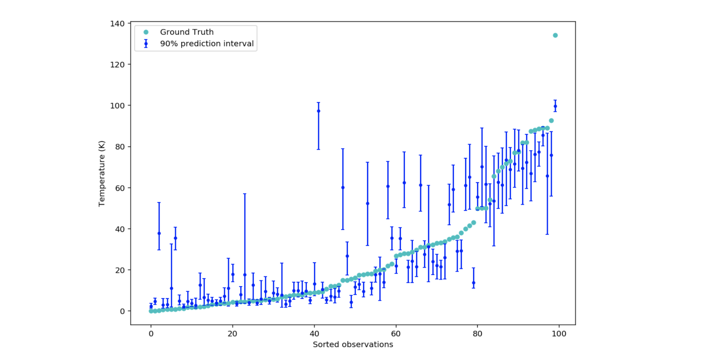 Figure 9: 90% prediction intervals with min_samples_leaf=100
When you repeat the counting procedure of fig. 6, only 54 out of 100 intervals contain the true critical temperature values. The result 0.54 no longer seems to be consistent with the expected probability 0.9.
However, we can overcome the problem by keeping in memory the values of each observation in the leaves (and not only their average) to rebuild the distribution of critical temperatures observed during training.
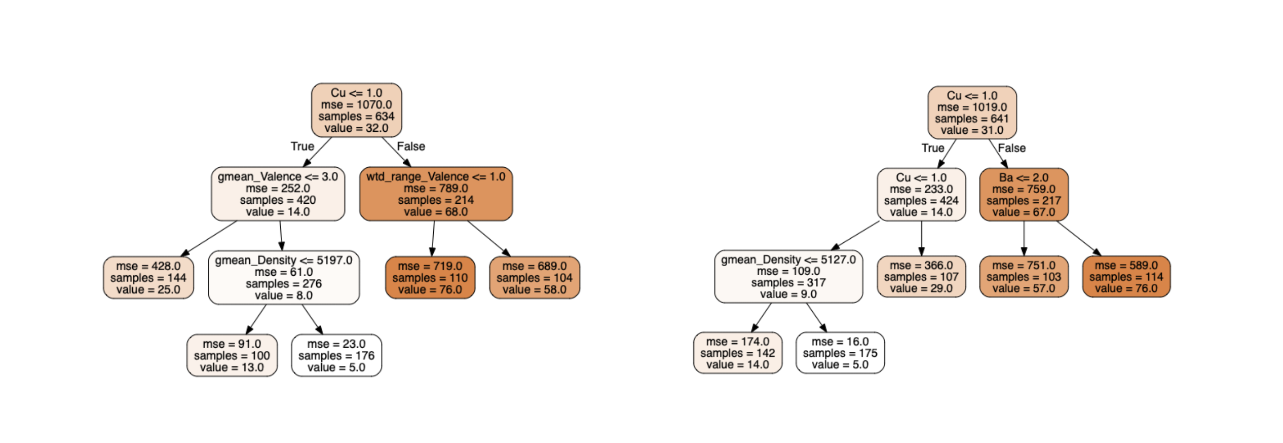 Figure 10: 2 trees with non-pure leaves
There are more than 100 samples of training data in the leaves. For the right leaf of the right tree, only the average of the 114 target values (76.0K) is stored. Nevertheless, the Quantile Regression Forest algorithm [3] keeps in memory each of the 114 critical temperatures associated with this leaf (and likewise for each leaf of each tree) in order to reconstruct the conditional distribution.
For one sample, the predicted distribution is computed by concatenating every values from every leaves in which the prediction falls with the associated weight.
With the fig. 10 example - a forest of two trees - if a sample fall in the left leaf of the left tree and the right leaf of the right tree, the stored values would be: $[y_{left-left-1}, y_{left-left-2}, …, y_{left-left-144}]$ weighted by $\frac{1}{144}$ and $[y_{right-right-1}, y_{right-right-2}, …, y_{right-right-114}]$ weighted by $\frac{1}{114}$.
The concatenation of all those weighted values then allows us to find the percentiles thanks to the weighted percentile method.
from skgarden import RandomForestQuantileRegressor

rfqr = RandomForestQuantileRegressor(criterion='mse', n_estimators=1000, min_samples_leaf=100)
rfqr.fit(X_train, y_train)

upper_prediction = rfqr.predict(X_test, quantile=95)
lower_prediction = rfqr.predict(X_test, quantile=5)
The code above build correct predicted distribution with pruned trees (min_samples_leaf=100). Around 90% of the intervals contains the true value.
Conclusion
Key takeaways:
-
A Random Forest delivers more information than one think
-
These are: quantify uncertainty, detect the region of additional measurements to make, find anomalies
-
Be sure not to build prediction intervals with too few trees (one need at least 100 points to describe the distribution)
To go further:
-
In classification, a probability is already an indicator of confidence (however, few algorithms deliver true probabilities, it is often necessary to calibrate them - this is the topic of the next article)
-
A technique that can work regardless of the model to find prediction intervals is the use of quantile loss to predict the conditional quantile $\alpha$ (two models need to be be trained - upper and lower percentile - to build the interval):
References
[1] A data-driven statistical model for predicting the critical temperature of a superconductor, Kam Hamidieh. 2018
[2] Random Forest, Leo Breiman. 2001
[3] Quantile Regression Forests, Nicolai Meinshausen. 2006
[4] https://blog.datadive.net/prediction-intervals-for-random-forests/
[5] https://scikit-garden.github.io/examples/QuantileRegressionForests/